


Modelling a pandemic: Symptomatic Isolation Policies - Part 1.
Part 5 of a layman's guide to modelling a pandemic.

Introduction.
This is the fifth in a series of articles introducing the Susceptible-Infectious-Recovered (S-I-R) compartmental model. This class of models was used by various expert groups to explore transmission dynamics and help decision-makers during the early stages of the Covid pandemic. The first four articles described the development of an S-I-R model that could be used to replicate the critical factors of viruses that lead to pandemic outbreaks.
The aim aim of these articles is to offer a guide for the layman, focusing on simplicity over technical complexity, hence any mathematics will be kept to a bare minimum. As in previous articles, I provide links to on-line models for you to explore. Interacting with these models is a very good way to understand them, and I would encourage you to experiment with the simple models through the links provided.
Summary
To recap, the first article introduced the S-I model, which demonstrated the driving force of exponential growth behind any pandemic contagion. The second article added the recovery phase to complete the simple S-I-R model and led to the important finding that population immunity, also known as 'herd' immunity, can halt an outbreak before infecting all susceptible individuals. Finally, the third article included an incubation phase, and the fourth article added asymptomatic transmission to the model. This completed the development an S-I-R model which could be easily adapted to represent different pandemic pathogens.
The S-I-R model we have developed so far has helped us understand fundamental forces driving the behaviour a pandemic. It can be thought of as an explanatory model. However, the true power of any modelling effort lies in the ability to test different policies that could be implemented to control a pandemic.
In this article, we will add a simple isolation policy to the S-I-R model. The policy will be to isolate individuals who are symptomatic and assess how well this works to contain outbreaks caused by pathogens with different characteristics. Different levels of the policy will be explored and measured against there ability to reduce the burden on the population, healthcare service, and economy.
Modelling a simple isolation policy
Isolation of infectious individuals remains an important method to control disease outbreaks. However, there are various ways to implement any isolation policy. In this article, we examine one of the simplest approaches - the isolation of symptomatic infectious individuals.
The following stock and flow diagram illustrates the S-I-R model updated to include the isolation of symptomatic infectious individuals.
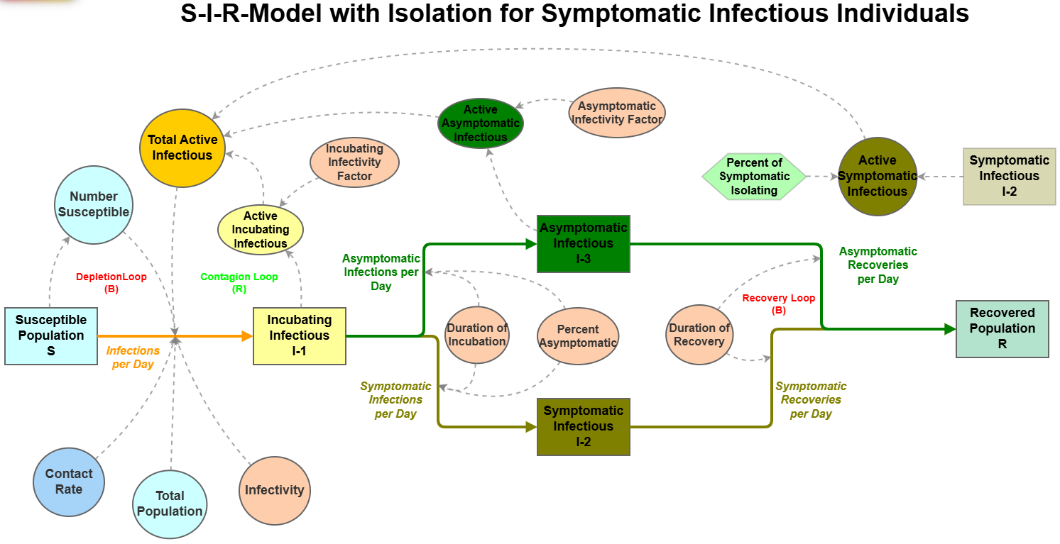
The isolation policy is represented in the diagram by the green hexagon variable called Percent of Symptomatic Isolating. This factor is applied to the number of individuals in the stock of Symptomatic Infectious I-2 to calculate the Active Symptomatic Infectious variable. When the Percent of Symptomatic Isolating policy variable is 100% then all symptomatic people isolate and when set to 0% none isolate. Values in between represent different strengths of the isolation policy modelled.
By now you will have seen that as a model becomes more complex, the number of connections between different components can start to become daunting. Links and Flows start to cross each other in many places leading to a "spaghetti"-like model appearance that can be difficult to follow. Ghosting is a tool that can be used to combat this graphical complexity and and the S-I-R stock and flow diagram shown above uses ghosting to simplify the picture.
The green hexagon Percent of Symptomatic Isolating variable is an example of a ‘ghost’ variable as it mirrors the value of the ‘master’ Percent of Symptomatic Isolating variable calculated in a separate part of the model. The following diagram depicts the logic used to set the Percent of Symptomatic Isolating variable in the model.
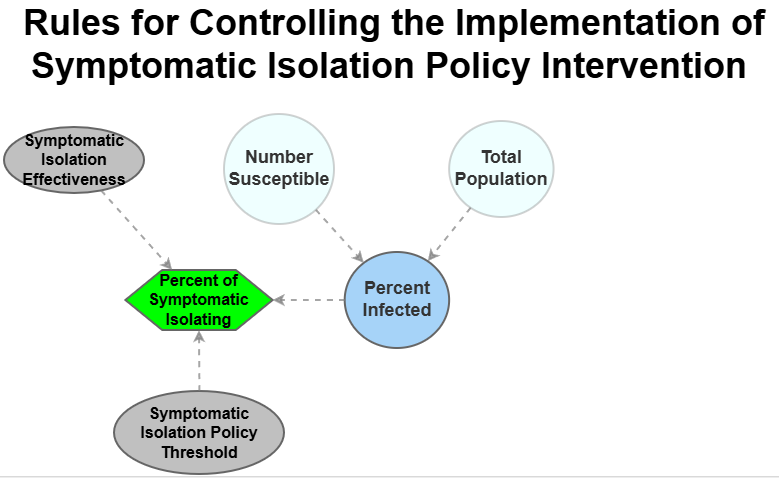
In this case, I have chosen to use the cumulative percent of the population infected as a threshold for when the policy is implemented. The diagram shows that the cumulative Percent Infected is calculated using the ghost variables Number Susceptible and Total Population from the S-I-R model. When the Percent Infected exceeds the Symptomatic Isolation Policy Threshold then the green Percent of Symptomatic Isolating policy variable is set to the Symptomatic Isolation Effectiveness variable which represents the expected percentage of symptomatic individuals that will isolate. If the percent of the population does not exceed the threshold then this policy variable is set to 0% and no symptomatic individuals isolate.
Separating the logic of the policy rules from the S-I-R transmission model is sound modelling practice, as it makes it easier to change policies in the model. For example, the timing for launching the policy could be adjusted to correspond to the number of days since the first infection is detected. Alternatively, the effectiveness of the policy could be modified to vary over time, reflecting an initial ramp-up period or a fall in public support.
With this simple policy for isolating symptomatic individuals implemented, we can now run the model to evaluate the likely impact of running the policy under different conditions. In the following sections we will look at the impact of changing the effectiveness of symptomatic isolation for viruses with different characteristics. But first we need to define the characteristics of our ‘virtual’ viruses and establish the measures we will use to assess the policy.
Defining the ‘virtual’ viruses.
As we have seen in previous articles, certain biological factors of pathogens make them more likely to create pandemics. In a 2012 paper that looked at the uncertainties surrounding a potential outbreak of pandemic influenza, the authors wrote:
Using sensitivity analysis we found that the most important disease characteristics are the fraction of transmission that occurs prior to symptoms, the reproduction number, and the length of each disease stage.
Using the S-I-R model we can create a number of ‘virtual’ pathogens where these disease characteristics vary. These ‘virtual’ pathogens can then be used to test how robust the different implementations of any policy for different viruses. To illustrate the principle we will use three ‘virtual’ pathogens that represent the original Covid strain, a novel pandemic Flu virus, and a novel persistent Covid virus.
The following table provides details of the values assigned in the model for each of the ‘virtual’ viruses that will be used to test the symptomatic isolation policies.

For all of the ‘virtual’ viruses, the reproduction number (R0) is 2.5, 30 percent of infections are asymptomatic, and the average number of daily contacts (the Contact Rate) is 11.
As you can imagine it is possible to configure a large number of 'virtual' viruses, requiring an element of judgment. In this case, I have chosen to use the original strain of Covid as a baseline virus. The Pandemic Flu virus has the same characteristics as seasonal flu but with higher infectivity, as we are using the same R0 value as Covid. The third 'virtual' virus modifies the original Covid virus by extending the duration of the symptomatic infectious period.
What does success look like?
The final step before using the model to test any policies is to define what success looks like. Once again it would be possible to use many different measures of success but for our purposes we will use the following three metrics.
Total number of people that get infected. This metric represents the burden of the disease on the population. For example, applying an infection fatality rate to this metric gives an indication of the number of fatalities. In addition, long-term health impacts (like Long Covid) could be estimated using this measure. Needless to say, the lower the number of people infected the better.
Daily trend of the number of symptomatic infectious people. This provides a measure of the likely impact on the health service in two ways. First, by applying an infection rate to this metric, it is possible to assess if health care capacity is likely to be exceeded at any time. Second, the timing of when the peak in this metric occurs provides insight into how long the health service has to prepare. The flatter and more delayed the trend for symptomatic infectious people, the better.
Total number of isolation days. This metric gives an indication of the negative economic impact or comparative benefit of each policy scenario. Here, we make the simple assumption that labour shortages from isolation are bad for GDP. The lower the number of days individuals isolate the better.
Modelling what happens with no isolation.
Before testing the effectiveness of different symptomatic isolation policies let’s first look at the success metrics for outbreaks of each ‘virtual’ virus without any isolation taking place. This will serve as a baseline to assess how well the policies perform. It also will show how viruses with the same reproduction number (R0) can have very different pandemic outbreak profiles.
If you would like to explore the enhanced model for these three ‘virtual’ viruses then click on the following link. As a reminder, Appendix 2 provides a guide to running the model.
The following chart plots the results of the model showing the population burden, as measured by the cumulative number of individuals that have been infected by day, for each of the three ‘virtual’ viruses assuming that no symptomatic individual isolates.
Whilst each virus follows a different trajectory the final number of infected people is identical with just under 90% of the population infected by day 180. This is because the three viruses have the same reproduction number (R0). However, Pandemic Flu has a shorter symptomatic period and higher infectivity during the incubation phase which drives the faster rate of climb. In contrast, Persistent Covid has the longest symptomatic period which gives a slower rate of climb.
The following chart illustrates this pattern by showing the number of infections per day for the three ‘virtual’ viruses.
At first sight this would indicate that Pandemic Flu presents the greatest problem for the healthcare system. However, plotting the number of symptomatic individuals per day for each virus presents a different picture as the following chart shows.
In contrast to the trends for infections per day, Persistent Covid with no one isolating presents a greater threat to the healthcare system albeit there is longer time to prepare for the peak in demand. This is because people with Persistent Covid are sicker for longer.
Testing the effectiveness of symptomatic isolation policies.
Having set a baseline, we can now develop a set of policy scenarios to test. For these ‘what if experiments’ we will assume that the policy is implemented when the first infected person arrives. However, the percent of symptomatic people that isolate will be changed to represent the strength of the policy and how well it is followed.
When determining the percent isolating, it is important to consider what happens during the course of an illness — some people may be mildly symptomatic and not recognise they are sick, whilst others may be more severely impacted but recover sufficiently to think they are no longer infectious. Consequently, it is very unlikely that it will be possible to isolate a symptomatic person immediately they show the first symptoms until they stop becoming infectious. Also the degree to which individuals are willing or able to isolate will vary — some will find it difficult without financial support, whilst some policies will provide full support. Finally, the strength with which a government enforces the policy has an impact.
For our set of policy experiments, we will run the model with a light-touch policy where 20% of symptomatic individuals isolating for the duration of their symptoms, a middle-ground policy with 50% isolating, and a very strict policy where 80% isolate.
The following table shows the burden on the population as measured by the number of people infected for each of the three ‘virtual’ viruses for light touch, middle ground and strict implementation of the policy to isolate symptomatic individuals.
The table shows that the light touch policy only has a small impact reducing the percent infected by about 5% for all of the the three virtual viruses from the ‘no isolation’ baseline model. Whilst increasing the strength of the symptomatic isolation policy does reduce the population burden it requires the strictest level of implementation of the policy to have a major impact. However, for the ‘virtual’ Pandemic Flu virus the strictest control level is still not sufficient to significantly reduce the population burden which remains at 60%.
The following panel charts show the impact on healthcare as measured by the number of symptomatic individuals per day for the same set of scenarios.
Again we can see that the isolation policies do reduce the impact on the health care system by ‘flattening’ the curve and delaying the peak. The impact is greatest for the Persistent Covid virtual virus where the impact can be completely mitigated, whereas Pandemic Flu continue to be a significant burden on the healthcare system even with the strictest controls.
Our final measure looks at the economic burden by comparing the total number of days lost through isolation for each of the three policies. The following table summarises the results for the same scenarios.
Unlike the previous measures, which progressively improved with increased isolation policy strength in all scenarios, the economic burden is highest for the 'middle ground' policy where 50% of the symptomatic population isolates for two of the virtual viruses. This reflects the longer symptomatic period defined for these two viruses and the need to move to the strongest level of policy control to control the outbreak.
In summary.
In this article we added the simplest control policy to the S-I-R model by isolating symptomatic individuals at three different levels of strength. The different control policies were tested with three ‘virtual’ variants that had different pandemic potential but had the same reproductive number (RO),
The model results showed that without isolation the ‘virtual’ Pandemic Flu virus with the shortest symptomatic period and highest infectivity during incubation was the most challenging virus to contain using symptomatic isolation.
In addition, only the strongest level of this isolation policy was able to stop the outbreak of any of the three ‘virtual’ variants.
Finally, the economic burden was highest when the policy was implemented at the middle ground level, indicating that it is better economically to go hard with any isolation policy.
This article looked at the impact of this simple isolation policy, assuming that it is implemented at the very start of the pandemic. However, in most cases this is impractical. In the next article we will examine how the timing for enacting the policy impacts the outcome.
Finally, although this article is longer than I intended I trust that you have found it of interest. As always, please ask any questions or leave your comments below.
Appendix 1. Sources
The following are links to the main source material used in this article.
Disease Outbreaks: Critical Biological Factors and Control Strategies
Kent Kawashima, Tomotaka Matsumoto, and Hiroshi Akashi. (2016)
Measuring the uncertainties of pandemic influenza
Jeanne Fair, et al. (2012)
Natalie Linton et al. (2020)
Appendix 2. Overview of the InsightMaker Interface
This section describes in more detail the InsightMaker screen interface using the enhanced S-I-R model as an example. The following image shows the landing page for the model. Click on the image and select full width from the … menu to view the detail.

The screen features three sections. The main portion of the screen presents a diagram depicting the model's logic as a stock and flow diagram. The boxes represent the population stocks which have different statuses These stocks are linked by flows, indicated by arrows, which move individuals from one stock to another at different rates. The circles/ellipses represent the variables of the model that are used to calculate the rates associated with the flows and control the model’s logic.
The right-hand panel has a dual function. The default setting, shown in the image above, displays information about the model and allows the user to adjust the values of some variables using sliders. It also allows you to choose from a set of scenarios that will automatically adjust the levels of the default settings. In this case the pre-set scenarios define the characteristics of the three ‘virtual’ viruses described in the main text above.
The second function is to allow the user to examine the model's logic in more detail. By selecting any of the stocks, flow rates, or variables, the panel shifts to present comprehensive information about the chosen building block. To revert to the default display, click anywhere on the main portion of the screen that is not a building block.
Finally, the area along the top of the screen allows the user to change the length of the simulation run and, most importantly, run the model by pressing the blue ‘SIMULATE’ button.
Thank you so much. This is fascinating and really helpful that you have presented it to those of us who might struggle. It makes a lot of sense but not sure how much the ‘powers that be’ would take the time and trouble to educate themselves in order to contribute to effective decision-making!
🙏