


Modelling a pandemic: Infection Matters
Part 3 of a layman's guide to modelling a pandemic.

Introduction.
This is the third in a series of articles introducing the Susceptible-Infectious-Recovered (S-I-R) compartmental model. This class of models was used by various expert groups to explore transmission dynamics and help decision-makers during the early stages of the Covid pandemic, most notably those from Imperial College. For newcomers to my Substack, the first article of the series is available here and the second article here.
The fourth article in the series exploring asymptomatic transmission can be found by clicking on the following button.
The aim is to offer a guide for the layman, focusing on simplicity over technical complexity, hence any mathematics will be kept to a bare minimum. As in previous articles, I will provide links to on-line models for you to explore. Interacting with these models is a very good way to understand them, and I would encourage you to experiment with the simple models through the links provided.
In this article we will focus on the infectious population and discuss the importance of the timeline of infectiousness and the onset of symptoms which plays a critical role in disease outbreaks and the policies required to bring them under control. The simple S-I-R model is enhanced to add an incubating population where individuals are infectious but do not exhibit symptoms. Finally, the impact of including an incubating population on the dynamics of a pandemic are explored using the enhanced model.
Recap.
The first article in this series on modelling a pandemic, focussed on the Susceptible-Infectious (S-I) component of the S-I-R model using a System Dynamics ‘Stock and Flow’ model. The model showed how the progress of an epidemic infection depends on the balance between a reinforcing contagion feedback loop and a balancing depletion loop.
In the second article, called ‘Time to Recover’, we completed the simple S-I-R model by adding the recovered population who after infection retained full immunity.
The following image shows the stock and flow diagram for the simple S-I-R model where a new stock called Recovered Population was added together with new flow called Recoveries per Day. These additions created a second balancing Recovery Loop that also acts as a brake on the reinforcing contagion loop.

By making these changes we found that the dynamics of the simple S-I-R model are altered, leading to the important finding that population immunity, also know as 'herd' immunity, can halt an outbreak before it infects all susceptible individuals. In addition, the model provided insights into the factors that lead to an epidemic, explaining why some infectious pathogens spread and some don’t.
In the following section we will explore why its important to model the infectious population in more detail to better represent the nature of many diseases.
Infectiousness and symptoms.
In situations where effective vaccines are not available, controlling an epidemic relies on safeguarding the susceptible population by preventing the spread of infection through contact. This usually involves promptly identifying and isolating infectious individuals, which can be challenging, particularly for a new infection where large-scale testing may not be feasible. In the absence of widespread testing, the emergence of symptoms becomes the primary method for identifying infectious individuals.
Identifying infectious individuals based on symptoms can be problematic for two reasons. Firstly, the infection may exhibit symptoms that are similar to those of other, less serious and more prevalent infections. This can hinder effective communication with the public and lead to confusion, which might result in infectious individuals not isolating as necessary. For instance, numerous symptoms of Covid are also found in other infections and may differ from person to person, creating ambiguity regarding who should isolate.
The second and potentially more serious challenge stems from the nature and timing of the ‘incubation period’. The incubation period of an infection refers to the time span from exposure to the onset of symptoms. The length of this period varies among diseases and is affected by several factors, such as the dose and method of infection, along with the host's vulnerability and reaction. During this period, an individual might be infectious, depending on the type of disease and their state of health.
The difference between the time when symptoms of an infection are observed and the period during which the individual is infectious is critical to consider in both prescribing infection control measures and modelling.
The following diagram illustrates three different timelines for incubation and the onset of symptoms. The red regions indicate periods when an individual is infectious, and blue regions denote the presence of symptoms. The orange diamond marks the point at which an individual could be isolated based on symptom onset.

The diagram shows that the timings can vary depending on the infectious disease. In the simplest case the entire time an infected individual is contagious occurs after the first symptoms appears and ends before the symptoms disappear. This Complete Overlap where all symptomatic individuals are infectious simplifies identification and makes control measures like quarantine and contact tracing more effective. SARS is an example of an infection that follows this pattern and it is likely that this helped contain the SARS pandemic. This timing pattern requires no change to the S-I-R model as the infectious population will all exhibit symptoms.
In contrast, diseases such as HIV/AIDS have completely different infectious and symptomatic periods. For diseases with No Overlap quarantine and contact tracing are less effective. Instead, prophylactic measures to reduce the pathogen's infectivity are implemented, such as promoting condom use to prevent HIV transmission. Modelling diseases with no overlap of infectiousness and symptom onset requires splitting the infectious population into incubating infectious and symptomatic infectious classes to more accurately reflect the nature of the disease.
In the two cases discussed so far the relationship between peak infectivity and symptomatic periods is clear. However, some diseases exhibit Partial Overlap of infectious and symptomatic periods, complicating the containment of outbreaks. For diseases with such overlapping periods, like pandemic influenza, a combination of strategies to diminish the pathogen's infectivity and to quarantine symptomatic individuals, as well as those exposed, is advisable.
The most effective modelling approach for diseases with partial overlap involves dividing the infectious group into two, similar to the approach for diseases without overlap. In the next section we will modify the simple S-I-R model to more accurately reflect diseases with no or partial overlap of the infectious and symptomatic states.
Enhancing the S-I-R model.
The previous section recommended that for certain diseases, the timeline of infectiousness and symptom onset would be more accurately depicted by dividing the infectious population into two distinct categories within the simple S-I-R model. The following diagram shows the Stock and Flow diagram where the infectious population is now represented by two new stocks and one new flow.

The new stocks are named Incubating Infectious I-1 and Symptomatic Infectious I-2, linked by a new flow called Symptomatic per Day. This new flow is calculated by dividing the count of individuals in the Incubating Infectious I-2 stock by the new variable, Duration of Infection, which has a default value of 5 days. This calculation doesn't mean that everyone incubates the disease for exactly 5 days; rather some people incubate faster and others slower, but the average is 5 days.
Finally, the reinforcing Contagion Loops are completed by summing the number of incubating infectious individuals with the number of symptomatic infectious individuals. This sum creates a new variable named Total Infectious, which is then used to calculate the Infections per Day flow using the same method applied in the simple S-I-R model.
The Recoveries per Day flow follows the calculation method used in the basic S-I-R model, maintaining a default duration of symptoms set at 5 days. Once again, this means that the recovery rate varies, with some individuals recuperating quicker and others taking longer than the average five-day period.
The inclusion of an incubation period in our simple S-I-R model has created two reinforcing contagion loops driven by the number of incubating infectious and symptomatic infectious individuals. In the next section we will see how this subtly changes the dynamics of a pandemic. The added incubation period has also increased the overall length of the infectious period. With the default settings of 5 days for the duration of both incubating and symptomatic states the infectiousness period has been doubled to 10 days. To account for this and remain consistent with the simple S-I-R model the default setting for Infectivity has been halved.
Running the enhanced S-I-R model.
Whilst the enhanced S-I-R model retains the same basic structure as the simple S-I-R model, adding the incubation period does change the dynamic behaviour of the model. This is because we now have two reinforcing contagion loops that are linked by the Symptomatic per Day flow between the Incubating Infectious and Symptomatic Infectious stocks . This is shown in the following image of the enhanced S-I-R model screen interface where the two reinforcing contagion loops are shown in green text.

The model's default settings assume a 5-day period for both incubation and symptom duration, totalling 10 days of infectiousness. However, what would happen if the incubation period were reduced to 0.5 days while maintaining the same overall infectiousness duration? And what would happen if the incubation period was increased to 9.5 days still keeping a total of 10 days for infectiousness?
The enhanced model allows us to explore these scenarios which can easily done by selecting one of the pre-set scenarios from the pull down menu in the right hand panel on the interface screen. You can run the model and asses the impact of these these three scenarios on the progress of the infections per day and recovered population by clicking on the following link.
A full description of how to run an InsightMaker model is provided in Appendix 2.
Running the model under these three distinct scenarios demonstrates the change in pandemic dynamics based on alterations to the incubation and symptomatic periods duration. The subsequent chart displays the model's results, depicting the trajectory of recovered individuals across the three scenarios. It is important to note that the model presumes the absence of any control measures.
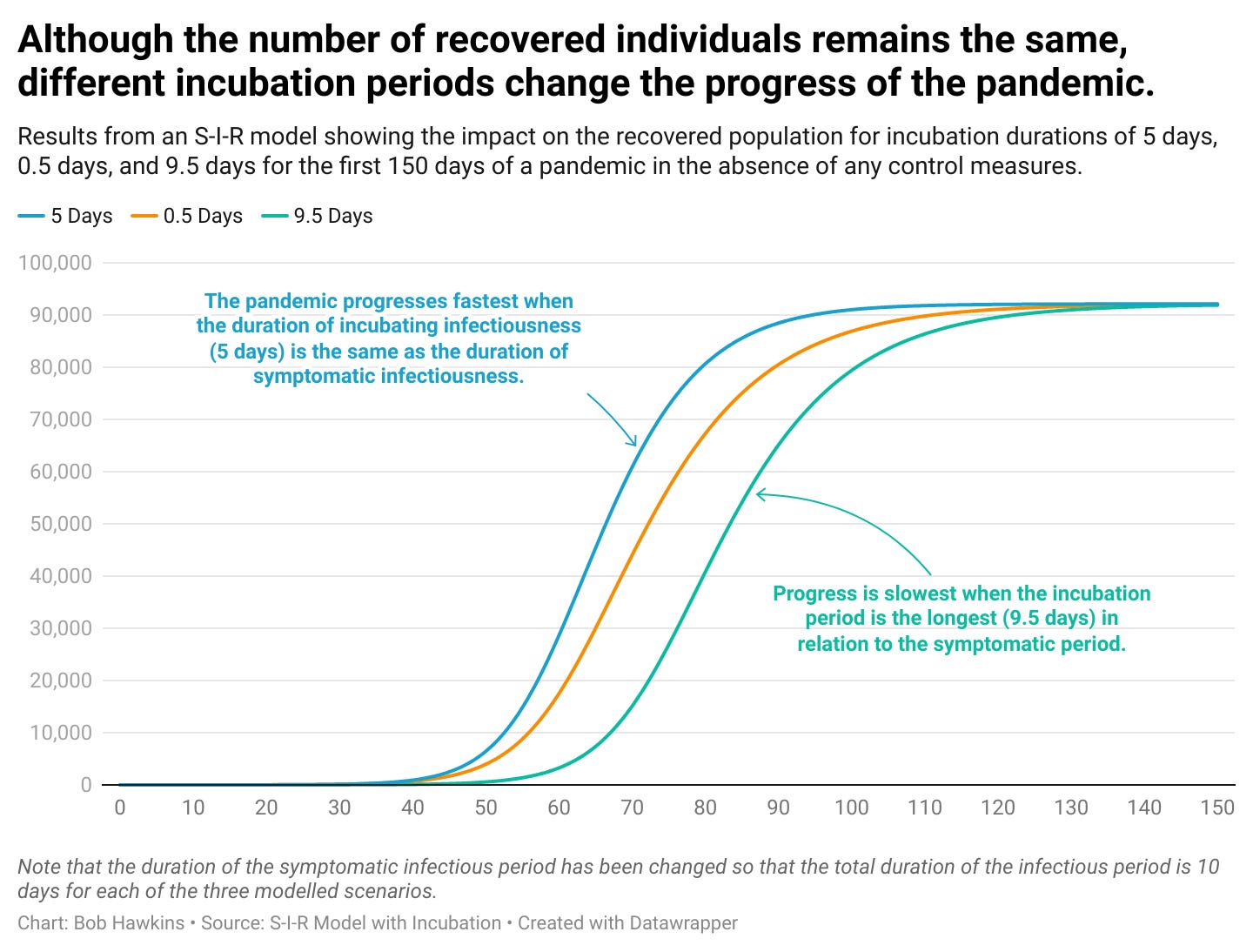
The first thing to note is that the number of individuals who have recovered by the end of the simulation is the same across all three scenarios. This indicates that the duration of the incubation period does not affect the level of population (‘herd’) immunity, as long as the total duration of the infectious period remains unchanged.
However, the path to population immunity varies with each scenario. The pandemic advances most rapidly when both the duration and the symptomatic period are set at five days. At this point, the two contagion loops are in balance. Moving away from this balance invariably leads to a slower progression of the pandemic, with the slowest rate of spread occurring when the incubation period is at its longest.
In conclusion.
In this article we explored how the nature of the overlap between incubation and the onset of symptoms is a critical factor in the development of disease outbreaks and can impact control strategies. In particular, control strategies that rely on the onset of symptoms to identify infectious individuals to quarantine are not as effective when there is a no overlap between incubation and symptomatic periods.
This implies that the S-I-R model should be enhanced to account for an incubation period during which individuals are infectious yet not showing any sings of symptoms. Incorporating this incubation period allows for the implementation of policies such as contact tracing, which aim to isolate those who are in the incubation phase of the infection, into the model.
The next article will examine some of the particular challenges posed by Covid, such as asymptomatic transmission, and will demonstrate how they can be modelled to allow the evaluation of different control policies.
Finally, I hope that you have found this article interesting and feel free to ask any questions or leave your comments below.
Appendix 1. Sources
The following are links to the main source material used in this article.
Disease Outbreaks: Critical Biological Factors and Control Strategies
Kent Kawashima, Tomotaka Matsumoto, and Hiroshi Akashi. (2016)
Factors that make an infectious disease outbreak uncontrollable
Christopher Fraser, Steven Riley, Roy M, Anderson, and Neil M. Ferguson. (2004)
Appendix 2. Overview of the InsightMaker Interface
This section describes in more detail the InsightMaker screen interface using the simple S-I model as an example. The following image shows the landing page for the model. Click on the image and select full width from the … menu to view the detail.

The screen features three sections outlined in red. The main portion of the screen presents a diagram depicting the model's logic as a stock and flow diagram. The two boxes are the susceptible and infectious population stocks, linked by a flow, indicated by a blue arrow, labelled 'Infections per Day'. The circles represent the variables of the model that determine the 'Infections per Day' rate.
The right-hand panel has a dual function. The default setting, shown in the image above, displays information about the model and allows the user to adjust the Contact Rate or Infectivity using sliders. It also allows you to choose from a set of scenarios that will automatically adjust the levels of the default settings.
The second function is to allow the user to examine the model's logic in more detail. By selecting any of the stocks, flow rates, or variables, the panel shifts to present comprehensive information about the chosen building block. To revert to the default display, click anywhere on the main portion of the screen that is not a building block.
Finally, the area along the top of the screen allows the user to change the length of the simulation run and, most importantly, run the model by pressing the blue ‘SIMULATE’ button.